Get started with jointVIP

install.packages("jointVIP")

The purpose of the jointVIP

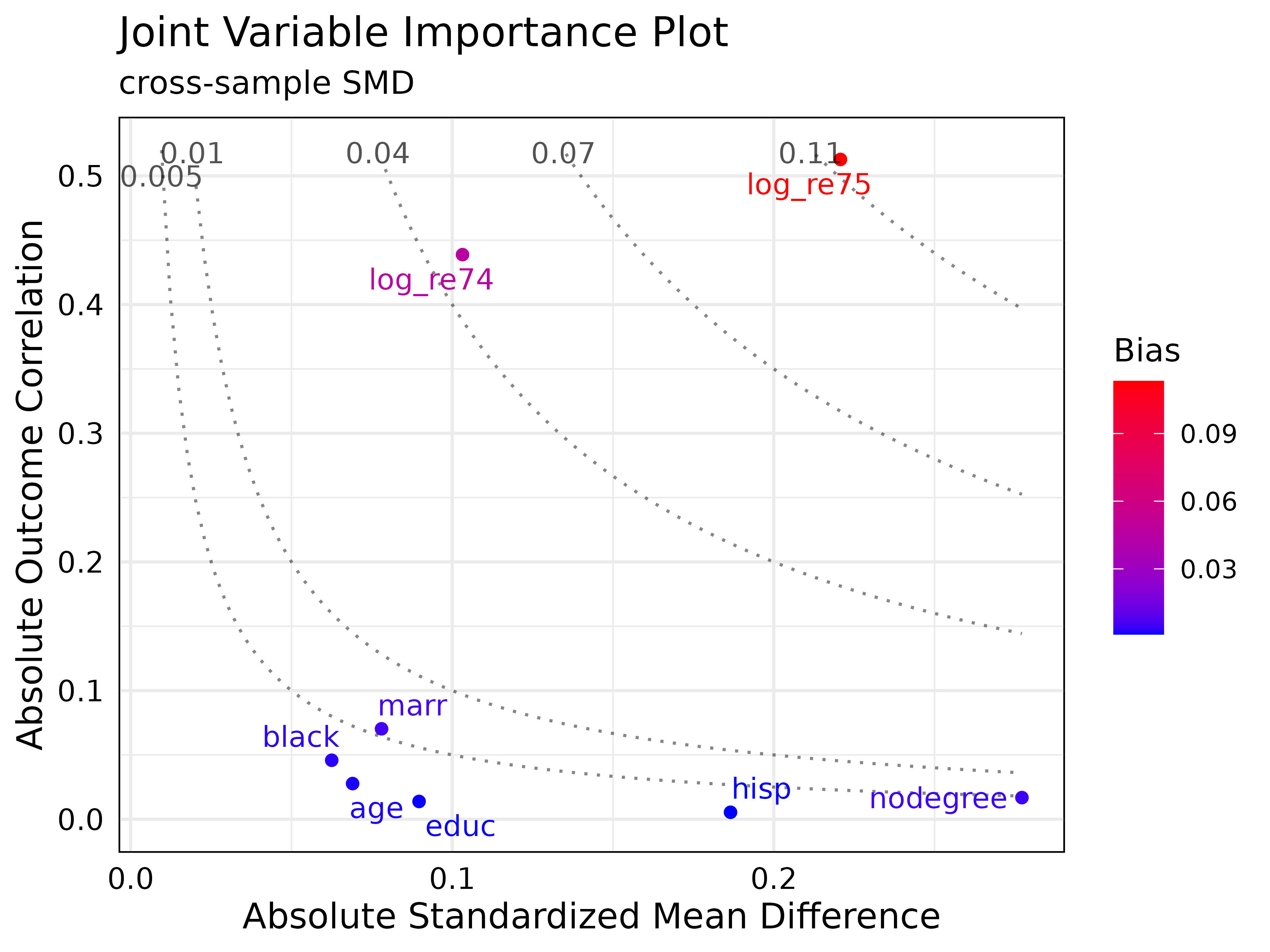
The joint variable importance plot (jointVIP for short) is designed to help identify which variables to prioritize based on both treatment and outcome for adjustment. This plot should be used during the design stage of the observational study prior to the analysis phase.

Traditionally, balance tables and Love plots are used to show standardized mean differences and identify variables with high treatment imbalance. However, adjusting only based on treatment imbalance is not advised since they may not be confounders. The jointVIP helps researchers prioritize variables that contribute marginal bias on both dimensions that can be used in observational study design. Additionally, bias curves based on simple one variable (unadjusted) omitted variable bias framework are plotted for the ease of comparison.

Set up for example

You can install the released version of jointVIP with:

# install once its on CRAN!
# install.packages("jointVIP")

# devtools::install_github("ldliao/jointVIP")

# load jointVIP package
library(jointVIP)

# data to use for example
library(causaldata)

# matching method shown in example
library(MatchIt)
library(optmatch)

# weighting method shown in example
library(WeightIt)
library(optweight)

Data cleaning

The example data uses data from the causaldata package, specifically the cps_mixtape and nsw_mixtape datasets (Huntington-Klein and Barrett 2021). The experimental version of the nsw_mixtape is commonly known as lalonde and often an example that shows propensity score matching, with propensity score estimated from the cps_mixtape data (Dehejia and Wahba 1999; LaLonde 1986).

Data set contains the following variables:

treat denoting whether the person was selected in the National Supported Work Demonstration job-training program
age age in years
educ years of education
black whether the race of the person was Black
hisp whether the ethnicity of the person was Hispanic
marr whether the person was married
nodegree whether the person has degree or not
re74 real earnings in 1974
re75 real earnings in 1975
re78 outcome of interest: real earnings in 1978

Here simple data cleaning is performed to log-transform the earnings. To avoid errors, those who earned 0 is transformed as $log(1) = 0$ . After transformation, the both data has new variables:

log_re74 log-real earnings in 1974
log_re75 log-real earnings in 1975
log_re78 outcome of interest: log-real earnings in 1978

The jointVIP package uses pilot_df and analysis_df to denote datasets used. The analysis_df is the matching/weighting dataset of interest while pilot_df contains the external controls not used in the analysis. The pilot_df is used to help inform the outcome correlation and compare the cross-sample standardized mean difference. If external data is not available, one may choose to sacrifice a portion of the analysis controls to form the pilot_df.

# load data for estimating earnings from 1978
# treatment is the NSW program
pilot_df = cps_mixtape
analysis_df = nsw_mixtape

transform_earn <- function(data, variables){
  data = data.frame(data)
  log_variables = sapply(variables, 
                         function(s){paste0('log_',s)})
  data[,log_variables] =
    apply(data[,variables], 2, 
        function(x){ifelse(x == 0, 
                           log(x + 1), 
                           log(x))})
  return(data)
}

pilot_df <- cps_mixtape
pilot_df <- transform_earn(pilot_df, c('re74', 're75', 're78'))

analysis_df <- nsw_mixtape
analysis_df <- transform_earn(analysis_df, c('re74', 're75', 're78'))

Specifying parameters for the `create_jointVIP()` function

To visualize for the jointVIP, following parameters must be specified:

treatment the treatment variable name; 0 for control and 1 for treated
outcome the outcome of interest
covariates covariates of interest that are common for the two pilot_df and analysis_df — the variables all should occur prior to treatment and be potential confounders
pilot_df pilot dataset consists of external controls
analysis_df analysis dataset consists of both treated and controls of interest

The new_jointVIP is a jointVIP object.

treatment = 'treat'
outcome = 'log_re78'
covariates = c(names(analysis_df)[!names(analysis_df) %in% c(treatment,
                                           outcome, "data_id",
                                           "re74", "re75",
                                           "re78")])

new_jointVIP = create_jointVIP(treatment = treatment,
                               outcome = outcome,
                               covariates = covariates,
                               pilot_df = pilot_df,
                               analysis_df = analysis_df)

Diagnostics with a `jointVIP` object

The summary() function outputs the maximum absolute bias, the number of variables are above the desired bias tolerance (measured in absolute always), and the number of variables that can be plotted.

summary(new_jointVIP, 
        smd = "cross-sample",
        use_abs = TRUE,
        bias_tol = 0.01)
#> Max absolute bias is 0.113
#> 2 variables are above the desired 0.01 absolute bias tolerance
#> 8 variables can be plotted

The print() function outputs the variables and its associated bias above the absolute bias_tol desired.

print(new_jointVIP,
      smd = "cross-sample",
      use_abs = TRUE,
      bias_tol = 0.01)
#>           bias
#> log_re75 0.113
#> log_re74 0.045

plot(new_jointVIP)

By visualizing with the jointVIP, several important aspects stand out. First, the most important variables are the log_re75 and log_re74. Traditional methods, such as the Love plot or balance table would indicate nodegree and hisp variables to be more important to adjust than log_re74, but these variables show low marginal bias contribution using the jointVIP.

Matching examples

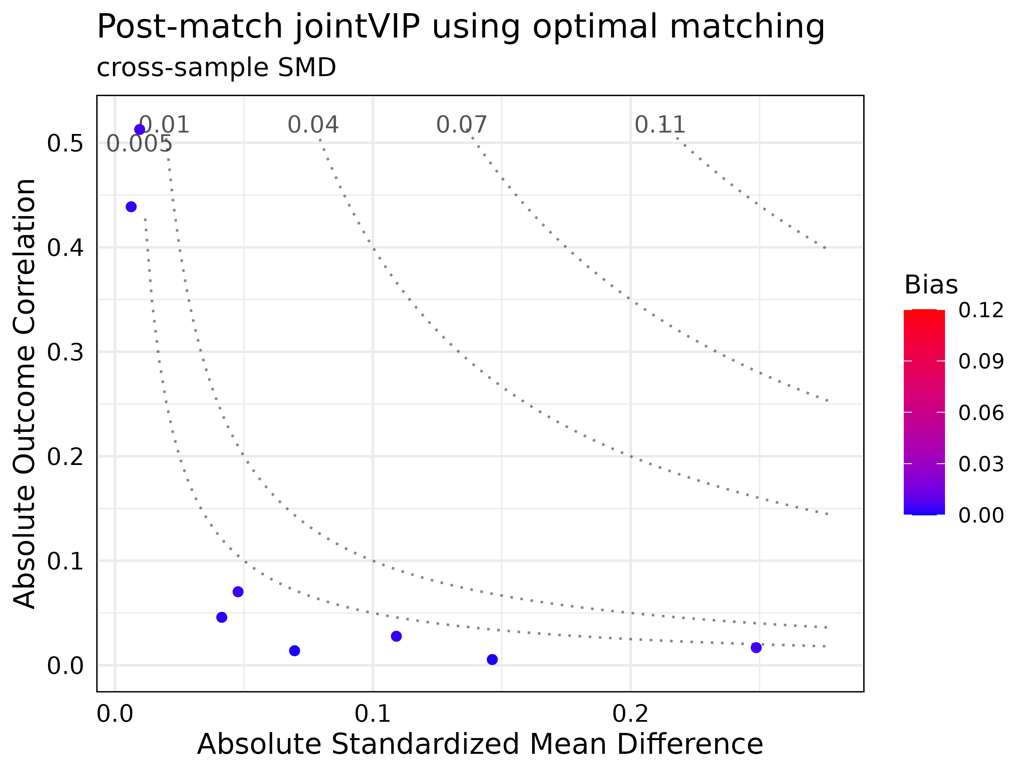
Following matching examples are performed to illustrate the utility of the jointVIP. Based on the plot shown above, the only variables that need adjustment are the log_re75 and log_re74. Post-match results are plotted to help visualize for comparison.

Optimal pair matching

As a simple example, optimal pair matching using Mahalanobis distance is used (Ho et al. 2011; Hansen 2007). Based on the desired bias tolerance, only log_re75 and log_re74 are inputted into the formula.

# 1:1 optimal matching w/o replacement
m.out <- matchit(
  treat ~ log_re75 + log_re74,
  data = analysis_df,
  method = "optimal",
  distance = "mahalanobis"
)
optmatch_df <- match.data(m.out)[, c(treatment, outcome, covariates)]

Optimal weighting

Optimal weighting example is performed below, basing the weights upon log_re75 and log_re74 (Greifer 2021). Please see documentation on Zubizarreta (2015) for details.

# ordering for the weightit
ordered_analysis_df = analysis_df[order(analysis_df$treat, decreasing = T),]

optwt <- weightit(treat ~ log_re74 + log_re75,
                  data = ordered_analysis_df,
                  method = "optweight", estimand = "ATE",
                  tols = 0.005, include.obj = TRUE)
# summary(optwt)

optwt_df = ordered_analysis_df[, c(covariates, treatment, outcome)]

Post-matching/weighting assessment with `post_jointVIP` object

Below are the examples showing how to plot after matching. The main function to use is the create_post_jointVIP() function, which takes in the original jointVIP object new_jointVIP in our example. The post-matched data frame need to be specified as post_analysis_df argument.

The functions: summary(), print(), and plot() all provide comparison between original and post jointVIPs. Note that the post-matched data frames contain the pair-matched individuals — for post-weighted data, an additional processing step multiplying the weight by the original data.frame subsetted on all the covariates.

All methods yielded satisfactory results based on desired bias tolerance.

post_optmatch_jointVIP <- create_post_jointVIP(new_jointVIP, 
                                               post_analysis_df = optmatch_df)

summary(post_optmatch_jointVIP)
#> Max absolute bias is 0.113
#> 2 variables are above the desired 0.01 absolute bias tolerance
#> 8 variables can be plotted
#> 
#> Max absolute post-bias is 0.005
#> Post-measure has 0 variable(s) above the desired 0.005 absolute bias tolerance
print(post_optmatch_jointVIP)
#>           bias post_bias
#> log_re75 0.113     0.005
#> log_re74 0.045     0.003
plot(post_optmatch_jointVIP, 
     plot_title = "Post-match jointVIP using optimal matching")

post_optwt_jointVIP = create_post_jointVIP(new_jointVIP,
                                           post_analysis_df = optwt_df,
                                           wts = optwt$weights)
summary(post_optwt_jointVIP)
#> Max absolute bias is 0.113
#> 2 variables are above the desired 0.01 absolute bias tolerance
#> 8 variables can be plotted
#> 
#> Max absolute post-bias is 0.005
#> Post-measure has 0 variable(s) above the desired 0.005 absolute bias tolerance
print(post_optwt_jointVIP)
#>           bias post_bias
#> log_re75 0.113     0.003
#> log_re74 0.045     0.003
plot(post_optwt_jointVIP, 
     plot_title = "Post-weighting jointVIP using optimal weighting")

References

Dehejia, Rajeev H, and Sadek Wahba. 1999. “Causal Effects in Nonexperimental Studies: Reevaluating the Evaluation of Training Programs.” Journal of the American Statistical Association 94 (448): 1053–62.

Greifer, Noah. 2021. WeightIt: Weighting for Covariate Balance in Observational Studies. https://CRAN.R-project.org/package=WeightIt.

Hansen, Ben B. 2007. “Optmatch: Flexible, Optimal Matching for Observational Studies.” New Functions for Multivariate Analysis 7 (2): 18–24.

Ho, Daniel E., Kosuke Imai, Gary King, and Elizabeth A. Stuart. 2011. “MatchIt: Nonparametric Preprocessing for Parametric Causal Inference.” Journal of Statistical Software 42 (8): 1–28. https://www.jstatsoft.org/v42/i08/.

Huntington-Klein, Nick, and Malcolm Barrett. 2021. Causaldata: Example Data Sets for Causal Inference Textbooks. https://CRAN.R-project.org/package=causaldata.

LaLonde, Robert J. 1986. “Evaluating the Econometric Evaluations of Training Programs with Experimental Data.” The American Economic Review, 604–20.

Zubizarreta, José R. 2015. “Stable Weights That Balance Covariates for Estimation with Incomplete Outcome Data.” Journal of the American Statistical Association 110 (511): 910–22.

Lauren D. Liao

2024-11-13

The purpose of the jointVIP

Set up for example

Data cleaning

Specifying parameters for the `create_jointVIP()` function

Diagnostics with a `jointVIP` object

Matching examples

Optimal pair matching

Optimal weighting

Post-matching/weighting assessment with `post_jointVIP` object

References

Get started with jointVIP

Lauren D. Liao

2024-11-13

The purpose of the jointVIP

Set up for example

Data cleaning

Specifying parameters for the create_jointVIP() function

Diagnostics with a jointVIP object

Matching examples

Optimal pair matching

Optimal weighting

Post-matching/weighting assessment with post_jointVIP object

References

Specifying parameters for the `create_jointVIP()` function

Diagnostics with a `jointVIP` object

Post-matching/weighting assessment with `post_jointVIP` object